This is a cheat sheet for Recurrent Neural Network learner, covers from math essentials of neural network to several different kinds of RNN. If you go through the whole content and understand thoroughly, you will at least be able to make your own neural network architecture, derive forward/backward propagation equations, which are fundamental to building your own working neural network.

Math Essentials

Notation	Meaning
a ∈ A	set membership
\| B \|	A cardinality: number of items in set B
\|\| v \|\|	norm: length of vector v
$\Sigma$	summation
$\int$	integral
$\Re$	the set of real numbers
$\Re^{n}$	real number space of dimension n n = 2 : plane or 2-space n = 3 : 3- (dimensional) space n > 3 : n-space or hyperspace
x, y, z, u, v	vector (bold, lower case)
A, B, X	matrix (bold, upper case)
$y=f(x)$	function(map):assigns unique value in range of y to each value in domain of x
$dy / dx$	derivative of y with respect to single
$y=f(x)$	function on multiple variables,i.e. a vector of variables; function in n-space
$∂y / ∂x_i$	partial derivative of y with respect to element i of vector x
$\|Ω\|$	the set of possible outcomes O
F	the set of possible events E
P	the probability distribution

Types of probability spaces

Define $\|Ω\|$; = number of possible outcomes

Discrete space $|Ω|$ is finite – Analysis involves summations $(∑)$

Continuous space $|Ω|$ is infinite – Analysis involves integrals $(∫)$

Expected value

Given:

A discrete random variable X, with possible values x = x1, x2, … xn
Probabilities $p( X = xi )$ that X takes on the various values of xi
A function $y_i = f( x_i )$ defined on X The expected value of f is the

probability-weighted “average” value of $f( x_i )$: $E( f ) = ∑_i p( x_i ) ⋅ f( x_i )$

Common form

\[μ =\frac{1}{N}∑_{i=1}^{n}x_i\]

Expected value in continuous spaces

\[E(f)=∫_{x=a→b} p(x)⋅f(x)\]

Variance

\[σ^2 = ∑_i p(x^i)⋅(x^i-μ)^2\]

Common form

\[σ^2=\frac{1}{N-1}∑_{i=1}^{n}(x_i−μ)^2\]

Covariance

\[cov(x,y)=∑_ip(x_i,y_i )⋅(x_i-μ_x )⋅(y_i -μ_y )\]

Common form

\[cov(x,y)=\frac{1}{N−1}∑_{i=1}^{n}(x_i −μ_x)(y_i −μ_y)\]

Correlation

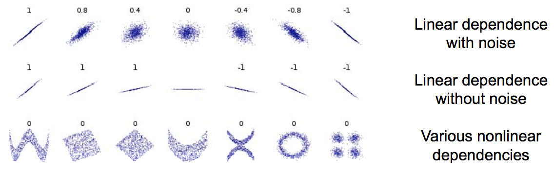
Pearson’s correlation coefficient is covariance normalized by the standard deviations of the two variables

\[corr(x, y)=\frac{cov(x, y)}{σ_xσ_y}\]

Always lies in range -1 to 1
Only reflects linear dependence between variables

Complement rule

Given: event A, which can occur or not

\[p( not A ) = 1 - p( A )\]

Product rule

Given: events A and B, which can co-occur (or not)

\[p( A, B ) = p( A \| B ) ⋅ p( B )\]

Rule of total probability

Given: events A and B, which can co-occur (or not)

\[p( A ) = p( A, B ) + p( A, not B )\]

Independence

Given: events A and B, which can co-occur (or not)

$p(A \| B)=p(A)$ or $p(A,B)=p(A)⋅p(B)$

Bayes rule

A way to find conditional probabilities for one variable when conditional probabilities for another variable are known.

posterior probability ∝ likelihood × prior probability

\[p( B \| A ) = p( A \| B ) ⋅ p( B ) / p( A )\]

where $p( A ) = p( A, B ) + p( A, not B )$

Some Linear algebra knowledge

Vector arithmetic

\[z=x+y=(x_1+y_1 ... x_n+y_n)^T\] \[y=ax=(ax_1 ... ax_n)^T\] \[a=x⋅y=∑_{i=1}^{n}x_iy_i\] \[a=x⋅y=||x||||y||cos(θ)\]

Matrix arithmetic

Multiplication is associative

$A ⋅( B ⋅ C ) = ( A ⋅B ) ⋅C$

Multiplication is not commutative

$A ⋅ B ≠ B ⋅ A$ (generally)

Transposition rule:

\[(A⋅B)^T =B^T ⋅A^T\]

Vector projection

Orthogonal projection of y onto x is the vector

\[proj_x(y) = x⋅\|\|y\|\|⋅cos(θ)/\|\|x\|\| =[(x⋅y)/\|\|x\|\|^2 ]x\]

(using dot product alternate form)

Stanford Machine Learning Tutorial:

Linear Regression

TODO

Nonlinear Regression

Sigmoid Function

\[P(y=1\|x)=h_θ(x)=\frac{1}{1+exp(−θ^⊤x)}≡σ(θ^⊤x)\] \[P(y=0\|x)=1−P(y=1\|x)=1−h_θ(x)\] \[\sigma(x)=\frac{1}{1+e^{-x}},x\in\mathbb{R}\] \[h_{\theta}(x)=\frac{1}{1+exp(−\theta^{⊤}x)}\]

Cost function

\[J(θ)=−∑_i(y^{(i)}log(h_θ(x^{(i)}))+(1−y^{(i)})log(1−h_θ(x^{(i)})))\]

Gradient

\[∇_θJ(θ)=\frac{∂J(θ)}{∂θ_j}=∑_ix^{(i)}_j(h_θ(x^{(i)})−y^{(i)})\]

Softmax Regression

\[h_θ(x)=\left[\begin{matrix}P(y=1|x;θ)\\P(y=2|x;θ)\\⋮\\P(y=K|x;θ)\end{matrix}\right]=\frac{1}{∑_{j=1}^Kexp(θ^{(j)⊤}x)}\left[\begin{matrix}exp(θ^{(1)⊤}x)\\exp(θ^{(2)⊤}x)\\⋮\\exp(θ^{(K)⊤}x)\end{matrix}\right]\] \[P(y^{(i)}=k|x^{(i)};θ)=\frac{exp(θ^{(k)⊤}x^{(i)})}{∑^{K}_{j=1}exp(θ^{(j)⊤}x^{(i)})}\]

Cost function (cross-entropy)

\[J(\theta)=-log(\frac { exp(w^T_jx) }{\sum^n_{i=1}exp(w^T_ix) } )=−w^T_jx+log(\sum^n_{i=1}exp(w^T_ix))\]

Gradient

\[∇_{θ^{(k)}}J(θ)=−∑_{i=1}^{m}\left[x^{(i)}(1\{y^{(i)}=k\}−P(y^{(i)}=k|;x^{(i)};θ))\right]\]

tanh

TODO

ReLU

TODO

TODO: more

RNN (Recurrent Neural Network)

LSTM

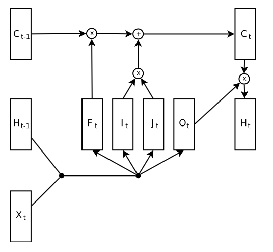
Overview of LSTM cell

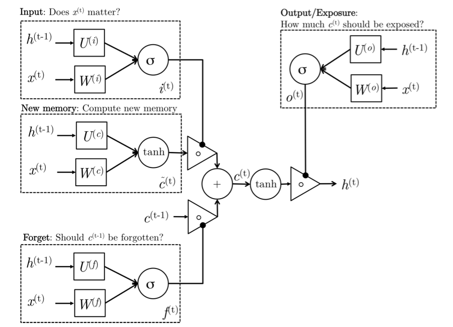
Details of LSTM cell

Intuition

New memory generation:This stage is analogous to the new memory generation stage we saw in GRUs. We essentially use the input word $x_t$ and the past hidden state $h_{t−1}$ to generate a new memory $\tilde{c_t}$ which includes aspects of the new word $x_{(t)}$.
Input Gate: We see that the new memory generation stage doesn’t check if the new word is even important before generating the new memory – this is exactly the input gate’s function. The input gate uses the input word and the past hidden state to determine whether or not the input is worth preserving and thus is used to gate the new memory. It thus produces it as an indicator of this information.
Forget Gate: This gate is similar to the input gate except that it does not make a determination of usefulness of the input word – instead it makes an assessment on whether the past memory cell is useful for the computation of the current memory cell. Thus, the forget gate looks at the input word and the past hidden state and produces $f_t$.
Final memory generation: This stage first takes the advice of the forget gate $f_t$ and accordingly forgets the past memory $c_{t−1}$. Similarly, it takes the advice of the input gate it and accordingly gates the new memory $\tilde{c_t}$. It then sums these two results to produce the final memory \(c_t$$.
Output/Exposure Gate: This is a gate that does not explicitly exist in GRUs. It’s purpose is to separate the final memory from the hidden state. The final memory $c_t$ contains a lot of information that is not necessarily required to be saved in the hidden state. Hidden states are used in every single gate of an LSTM and thus, this gate makes the assessment regarding what parts of the memory ct needs to be exposed/present in the hidden state ht. The signal it produces to indicate this is ot and this is used to gate the point-wise tanh of the memory.

Equations

$i_t = σ(W^{(i)}x_t + U^{(i)}h_{t−1})$ (Input gate)

$f_t = σ(W^{(f)}x_t + U^{(f)}h_{t−1})$ (Forget gate)

$o_t = σ(W^{(o)}x_t + U^{(o)}h_{t−1})$ (Output/Exposure gate)

$\tilde{c_t} = tanh(W^{(c)}x_t + U^{(c)}h_{t−1})$ (New memory cell)

$c_t = f_t ◦ c_{t−1} + i_t ◦ \tilde{c_t}$ (Final memory cell)

\[h_t =o_t◦tanh(c_t)\]

How LSTM backward propagation works?

Here’s a slide explaining this: LSTM Forward and Backward Pass

GRU

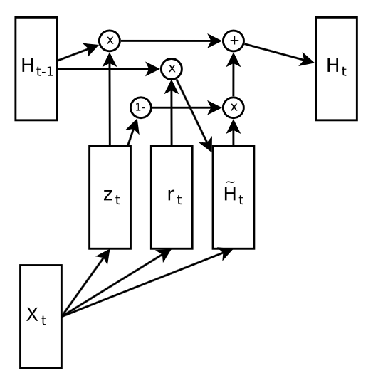
Overview of GRU cell

Details of GRU cell

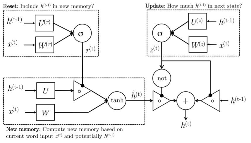
Intuition

New memory generation: A new memory $\tilde{h_t}$ is the consolidation of a new input word $x_t$ with the past hidden state $h_{t−1}$. Anthropomorphically, this stage is the one who knows the recipe of combining a newly observed word with the past hidden state $h_{t−1}$ to summarize this new word in light of the contextual past as the vector $\tilde{h_t}$.
Reset Gate: The reset signal $r_t$ is responsible for determining how important $h_{t−1}$ is to the summarization $\tilde{h_t}$. The reset gate has the ability to completely diminish past hidden state if it finds that $h_{t−1}$ is irrelevant to the computation of the new memory.
Update Gate: The update signal $z_t$ is responsible for determining how much of $h_{t−1}$ should be carried forward to the next state. For instance, if $z_t ≈ 1$, then $h_{t−1}$ is almost entirely copied out to ht. Conversely, if $z_t ≈ 0$, then mostly the new memory $\tilde{h_t}$ is forwarded to the next hidden state.
Hidden state: The hidden state ht is finally generated using the past hidden input $h_{t−1}$ and the new memory generated $\tilde{h_{t-1}}$ with the advice of the update gate.

Equations

$r_t = sigm (W_{xr}x_t + W_{hr}h_t−1 + b_r)$ (Reset gate)

$z_t = sigm(W_{xz}x_t + W_{hz}h_t−1 + b_z)$ (Update gate)

$\tilde{h_t} = tanh(W_{xh}x_t + W_{hh}(r_t ⊙ h_{t−1}) + b_h)$ (New memory)

$h_t = z_t ⊙h_{t−1} +(1−z_t)⊙\tilde{h_t}$ (Hidden state)

TODO: more RNN network and math

Thanks to

Jeff Howbert for his lecture note summarizing Machine Learning Math Essentials: Washington University CSS490 Winter 2012 lecture slide
Computer Science Department, Stanford University for their Deep Learning Tutorial: Stanford Machine Learning Tutorial
Nal Kalchbrenner, Ivo Danihelka, Alex Graves for their paper: Grid Long Short-Term Memory
Rafal Jozefowicz, Wojciech Zaremba and Ilya Sutskever for their paper: An Empirical Exploration of Recurrent Network Architectures
Christopher Olah for his clear explanation of LSTM: Understanding LSTM Networks
Andrej Karpathy for his post: The Unreasonable Effectiveness of Recurrent Neural Networks and excellent char-rnn code
Arun Mallya for his explanation how LSTM backward propagation works: LSTM Forward and Backward Pass