Statistics Reasoning by CMU
There are two version of this course in CMU, the other one is “Probability & Statistics”, I prefer this version because the “probability” part in this version acts as a “bridge” to the inference section thus making easier to understand and grab the big picture.
- UNIT 1
- UNIT 2: Exploratory Data Analysis:
- UNIT 3: Producing Data:
- UNIT 4: Probability:
- UNIT 5: Inference:
UNIT 1
The Big Picture
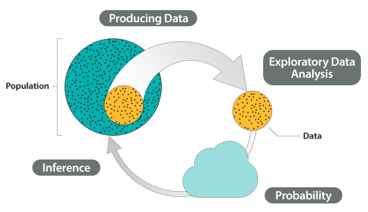
Producing data is choosing a sample and collecting data from it.
Inference is that we use what we’ve discovered about our sample to draw conclusion about our population.
Example
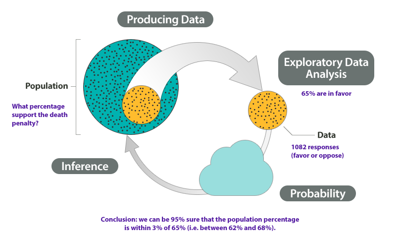
At the end of April 2005, a poll was conducted (by ABC News and the Washington Post) for the purpose of learning the opinions of U.S. adults about the death penalty.
The 4-step process
-
Producing Data: A (representative) sample of 1,082 U.S. adults was chosen, and each adult was asked whether he or she favored or opposed the death penalty.
-
Exploratory Data Analysis (EDA): The collected data were summarized, and it was found that 65% of the sampled adults favor the death penalty for persons convicted of murder.
-
and 4. Probability and Inference: Based on the sample result (of 65% favoring the death penalty) and our knowledge of probability, it was concluded (with 95% confidence) that the percentage of those who favor the death penalty in the population is within 3% of what was obtained in the sample (i.e., between 62% and 68%). The following figure summarizes the example:
UNIT 2: Exploratory Data Analysis:
Module 4: Examining Distributions
Distribution means:
- What values the variable takes
- How often the variable takes those values
Categorical distribution often uses pie-chart and bar-chart. Quantitative distribution often uses histogram, stemplot, boxplot.
When describing a distribution of quantitative variable, you need to include shape (symmetry, or skewed left, skewed right, Peakedness/modality—the number of peaks/modes the distribution has), center, spread (range), outliers.
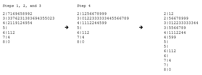
There is an interesting kind of plot sililar to histogram, stemplot.To make a stemplot:
- Separate each observation into a stem and a leaf.
- Write the stems in a vertical column with the smallest at the top, and draw a vertical line at the right of this column.
- Go through the data points, and write each leaf in the row to the right of its stem.
- Rearrange the leaves in an increasing order.
Measures of center
- The three main numerical measures for the center of a distribution are the mode, mean (\(\bar{x}\)), and the median (M). The mode is the most frequently occurring value. The mean is the average value, while the median is the middle value.
- The mean is very sensitive to outliers (because it factors in their magnitude), while the median is resistant to outliers.
- The mean is an appropriate measure of center only for symmetric distributions with no outliers. In all other cases, the median should be used to describe the center of the distribution.
Three most commonly used measures of spread
- Range
- Inter-quartile range (IQR)
- Standard deviation
The 1.5(IQR) Criterion for Outliers
An observation is considered suspected outlier if it is below Q1-1.5IQR or above Q3+1.5IQR.
Several possibilities about outliers
- Even though it is an extreme value, if an outlier can be understood to have been produced by essentially the same sort of physical or biological process as the rest of the data, and if such extreme values are expected to eventually occur again, then such an outlier indicates something important and interesting about the process you’re investigating, and it should be kept in the data.
- If an outlier can be explained to have been produced under fundamentally different conditions from the rest of the data (or by a fundamentally different process), such an outlier can be removed from the data if your goal is to investigate only the process that produced the rest of the data.
- An outlier might indicate a mistake in the data (like a typo, or a measuring error), in which case it should be corrected if possible or else removed from the data before calculating summary statistics or making inferences from the data (and the reason for the mistake should be investigated).
Choosing Numerical Summaries
Use \(\bar{x}\) (the mean) and the standard deviation as measures of center and spread only for reasonably symmetric distributions with no outliers.
Use the five-number summary (which gives the median, IQR and range) for all other cases.
Module 5: Examining Relationships
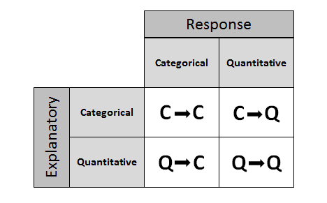
Four possibilities for role-type classification and corresponding data display and numerical summaries
-
Categorical explanatory and quantitative response
Data display: Side-by-side boxplots
Numerical summaries: Descriptive statistics
-
Categorical explanatory and categorical response
Data display: Two-way table, supplemented by
Numerical summaries: Conditional percentages.
-
Quantitative explanatory and quantitative response
Data display: Scatterplot
Numerical summaries: Use Correlation Coefficient to describe direction, form and strength, and least-square regression line (including intercept and slope) to accurate describe the pattern of data points.
A special case of the relationship between two quantitative variables is the linear relationship. In this case, a straight line simply and adequately summarizes the relationship.
When the scatterplot displays a linear relationship, we supplement it with the correlation coefficient (r), which measures the strength and direction of a linear relationship between two quantitative variables. The correlation ranges between -1 and 1. Values near -1 indicate a strong negative linear relationship, values near 0 indicate a weak linear relationship, and values near 1 indicate a strong positive linear relationship.
The correlation is only an appropriate numerical measure for linear relationships, and is sensitive to outliers. Therefore, the correlation should only be used as a supplement to a scatterplot (after we look at the data).
The most commonly used criterion for finding a line that summarizes the pattern of a linear relationship is “least squares.” The least squares regression line has the smallest sum of squared vertical deviations of the data points from the line.
The slope of the least squares regression line can be interpreted as the average change in the response variable when the explanatory variable increases by 1 unit.
The least squares regression line predicts the value of the response variable for a given value of the explanatory variable. Extrapolation is prediction of values of the explanatory variable that fall outside the range of the data. Since there is no way of knowing whether a relationship holds beyond the range of the explanatory variable in the data, extrapolation is not reliable, and should be avoided.
-
Quantitative explanatory and categorical response
This course didn’t discuss this topic, let me guess,
Data display: clustered scatterplot
Numerical summaries: Decision tree or Machine Learning methods (Softmax, etc.)
Causation and Lurking variables
An important principle: Association does not imply causation!
A lurking variable is a variable that was not included in the analysis, but that could substantially change the interpretation if it was included.
Whenever including lurking variables cause the change of the direction of an association, this is call Simpson’s Paradox.
UNIT 3: Producing Data:
Module 6: Sampling
Suppose you want to determine the musical preferences of all students at your university, based on a sample of students. Here are some examples of the many possible ways to pursue this problem.
-
volunteer sample
Post a music-lovers’ survey on a university IInternet bulletin board, asking students to vote for their favorite type of music.
Such a sample is almost guaranteed to be biased, we cannot generalize to any larger group at all.
-
convenience sample
Stand outside the Student Union, across from the Fine Arts Building, and ask students passing by to respond to your question about musical preference.
There are often subtle reasons why the sample’s results are biased.
-
sampling frame
Ask your professors for email rosters of all the students in your classes. Randomly sample some addresses, and email those students with your question about musical preference.
There may be bias arising because of this discrepancy.
-
systematic sampling
Obtain a student directory with email addresses of all the university’s students, and send the music poll to every 50th name on the list.
Systematic sampling may not be subject to any clear bias, but it would not be as safe as taking a random sample.
-
simple random sample
Obtain a student directory with email addresses of all the university’s students, and send your music poll to a simple random sample of students. As long as all of the students respond, then the sample is not subject to any bias, and should succeed in being representative of the population of interest.
Any plan that relies on random selection is called a probability sampling plan (or technique). The following three probability sampling plans are among the most commonly used:
-
Simple Random Sampling is, as the name suggests, the simplest probability sampling plan. It is equivalent to “selecting names out of a hat.” Each individual as the same chance of being selected.
-
Cluster Sampling—This sampling technique is used when our population is naturally divided into groups (which we call clusters). For example, all the students in a university are divided into majors; all the nurses in a certain city are divided into hospitals; all registered voters are divided into precincts (election districts). In cluster sampling, we take a random sample of clusters, and use all the individuals within the selected clusters as our sample. For example, in order to get a sample of high-school seniors from a certain city, you choose 3 high schools at random from among all the high schools in that city, and use all the high school seniors in the three selected high schools as your sample.
-
Stratified Sampling—Stratified sampling is used when our population is naturally divided into sub-populations, which we call stratum (plural: strata). For example, all the students in a certain college are divided by gender or by year in college; all the registered voters in a certain city are divided by race. In stratified sampling, we choose a simple random sample from each stratum, and our sample consists of all these simple random samples put together. For example, in order to get a random sample of high-school seniors from a certain city, we choose a random sample of 25 seniors from each of the high schools in that city. Our sample consists of all these samples put together.
Each of those probability sampling plans, if applied correctly, are not subject to any bias, and thus produce samples that represent well the population from which they were drawn.
random_sample = population[sample(length(population$Course),192),];random_sample
random_sample_percent = 100*summary(random_sample$Handed)/length(random_sample$Handed);
random_sample_percent;
pop_percent = 100*summary(population$Handed)/length(population $Handed);
pop_percent;
par(mfrow=c(1,2)); pie(pop_percent,labels=paste(c("left=","right="),round(pop_percent,0),"%"),main="Population");
pie(random_sample_percent,labels=paste(c("left=","right="),round(random_sample_percent,0),"%"),main="Random Sample")
summary(population$Verbal)
summary(random_sample$Verbal)
Module 7: Designing Studies
- Recruit participants for a study. While they are presumably waiting to be interviewed, half of the individuals sit in a waiting room with snacks available and a TV on. The other half sit in a waiting room with snacks available and no TV, just magazines. Researchers determine whether people consume more snacks in the TV setting.
This is an experiment, because the researchers take control of the explanatory variable of interest (TV on or not) by assigning each individual to either watch TV or not, and determine the effect that has on the response variable of interest (snack consumption).
- Recruit participants for a study. Give them journals to record hour by hour their activities the following day, including when they watch TV and when they consume snacks. Determine if snack consumption is higher during TV times.
This is an observational study, because the participants themselves determine whether or not to watch TV. There is no attempt on the researchers’ part to interfere.
- Recruit participants for a study. Ask them to recall, for each hour of the previous day, whether they were watching TV, and what snacks they consumed each hour. Determine whether snack consumption was higher during the TV times.
This is also an observational study; again, it was the participants themselves who decided whether or not to watch TV. Do you see the difference between 2 and 3? See the comment below.
- Poll a sample of individuals with the following question: While watching TV, do you tend to snack: (a) less than usual; (b) more than usual; or (c) the same amount as usual?
This is a sample survey, because the individuals self-assess the relationship between TV watching and snacking.
We will begin by using the context of this smoking cessation example to illustrate the specialized vocabulary of experiments. First of all, the explanatory variable, or factor, in this case is the method used to quit. The different imposed values of the explanatory variable, or treatments (common abbreviation: ttt), consist of the four possible quitting methods. The groups receiving different treatments are called treatment groups. The group that tries to quit without drugs or therapy could be called the control group—those individuals on whom no specific treatment was imposed. Ideally, the subjects (human participants in an experiment) in each treatment group differ from those in the other treatment groups only with respect to the treatment (quitting method).
# https://oli.cmu.edu/jcourse/workbook/activity/page?context=fbe0d83b0a0001dc429ce613d9a7112e
random_sample = computers[sample(length(computers$age), 450),]
group = sample(1:3,450,replace=T)
random_sample = cbind(random_sample,group)
boxplot(random_sample$age~random_sample$group, xlab="Group", ylab="Age (years)")
two_way_table = table(random_sample$group,random_sample$gender)
prop.table(two_way_table,1)*100
If neither the subjects nor the researchers know who was assigned what treatment, the experiment is called double blind.
Summary:
Observational studies:
-
The explanatory variable’s values are allowed to occur naturally.
-
Because of the possibility of lurking variables, it is difficult to establish causation.
-
If possible, control for suspected lurking variables by studying groups of similar individuals separately.
-
Some lurking variables are difficult to control for; others may not be identified.
Experiments
-
The explanatory variable’s values are controlled by researchers (treatment is imposed).
-
Randomized assignment to treatments automatically controls for all lurking variables.
-
Making subjects blind avoids the placebo effect.
-
Making researchers blind avoids conscious or subconscious influences on their subjective assessment of responses.
-
A randomized controlled double-blind experiment is generally optimal for establishing causation.
-
A lack of realism may prevent researchers from generalizing experimental results to real-life situations.
-
Noncompliance may undermine an experiment. A volunteer sample might solve (at least partially) this problem.
-
It is impossible, impractical or unethical to impose some treatments.
Examples:
Question: “What is your favorite kind of music?”
This is what we call an open question, which allows for almost unlimited responses. It may be difficult to make sense of all the possible categories and subcategories of music that survey respondents could come up with. Some may be more general than what you had in mind (“I like modern music the best”) and others too specific (“I like Japanese alternative electronic rock by Cornelius”). Responses are much easier to handle if they come from a closed question:
Question: Which of these types of music do you prefer: classical, rock, pop, or hip-hop?
What will happen if a respondent is asked the question as worded above, and he or she actually prefers jazz or folk music or gospel? He or she may pick a second-favorite from the options presented, or try to pencil in the real preference, or may just not respond at all. Whatever the outcome, it is likely that overall, the responses to the question posed in this way will not give us very accurate information about general music preferences. If a closed question is used, then great care should be taken to include all the reasonable options that are possible, including “not sure.” Also, in case an option was overlooked, “other:_______” should be included for the sake of thoroughness.
Many surveys ask respondents to assign a rating to a variable, such as in the following:
Question: How do you feel about classical music? Circle one of these: I love it, I like it very much, I like it, I don’t like it, I hate it.
Notice that the options provided are rather “top-heavy,” with three favorable options vs. two unfavorable. If someone feels somewhat neutral, they may opt for the middle choice, “I like it,” and a summary of the survey’s results would distort the respondents’ true opinions.
Some survey questions are either deliberately or unintentionally biased towards certain responses:
Question: “Do you agree that classical music is the best type of music, because it has survived for centuries and is not only enjoyable, but also intellectually rewarding? (Answer yes or no.)”
This sort of wording puts ideas in people’s heads, urging them to report a particular opinion. One way to test for bias in a survey question is to ask yourself, “Just from reading the question, would a respondent have a good idea of what response the surveyor is hoping to elicit?” If the answer is yes, then the question should have been worded more neutrally.
For the question, “Have you used illegal drugs in the past year?” respondents are told to flip a fair coin (in private) before answering and then answer based on the result of the coin flip: if the coin flip results in “Heads,” they should answer “Yes” (regardless of the truth), if a coin flip results in “Tails,” they should answer truthfully. Thus, roughly half of the respondents are “truth-tellers,” and the other half give the uncomfortable answer “Yes,” without the interviewer’s knowledge of who is in which group. The respondent who flips “Tails” and answers truthfully knows that he or she cannot be distinguished from someone who got “Heads” in the coin toss. Hopefully, this is enough to encourage respondents to answer truthfully. As we will learn later in the course, the surveyor can then use probability methods to estimate the proportion of respondents who admit they used illegal drugs in this scenario, while being unable to identify exactly which respondents have been drug abusers.
Summary
A sample survey is a type of observational study in which respondents assess variables’ values (often by giving an opinion).
- Open questions are less restrictive, but responses are more difficult to summarize.
- Closed questions may be biased by the options provided.
- Closed questions should permit options such as “other:__” and/or “not sure” if those options may apply.
- Questions should be worded neutrally.
- Earlier questions should not deliberately influence responses to later questions.
- Questions shouldn’t be confusing or complicated.
- Survey method and questions should be carefully designed to elicit honest responses if there are sensitive issues involved.
Lab Exercise
tbl = table(data.frame(data$Treat,data$Outcome)); tbl
100*tbl/rowSums(tbl)
plot(factor(data$Treat), data$Time)
tapply(data$Time, factor(data$Treat), summary)